1. The problem
1.1 One source, many consumers
Regardless of the application, every hydronic network is the same object: two collectors, a source that circulates the fluid between them, and a set of parallel branches that each take a share of the flow. A branch can be a radiator, a fan coil, an apartment riser, or a server bay. The requirement always boils down to: each branch must receive its design flow and maintain it regardless of the state of the other branches.
Two distinct failures lie behind this requirement. The static imbalance appears at the design point: when everything is working, the branch closest to the source receives more pressure than the furthest and therefore takes more flow. This is a distribution problem, resolved once during commissioning. The dynamic coupling appears during a change in configuration: when a branch closes or a pump switches, the total flow and pressure losses in the network change, and all the other branches diverge. It is a stability issue that determines the choice of the branch balancing device.
Only the permissible tolerance and the consequence of its exceedance change, depending on the application. In a dwelling, an underfed radiator results in a cold room. In a DLC network, insufficient flow causes throttling of a GPU: the guidelines aim for ± 5% on the branch flow, typically 1.5 L/min per kW for a temperature rise of about 10 °C (D2).
1.2 The physics of flow sharing
Let us take the example illustrated by Figure 1. The pumps create a Δpset that will balance with the downstream network; each branch only sees what remains after the distribution pressure loss. A branch is a radiator, a fan-coil unit, or a server bay.
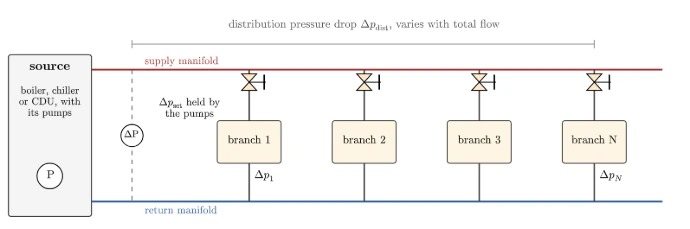
A branch equipped with a fixed adjustment device behaves like a hydraulic resistance. Its flow rate is governed by the branch law:
ṁj = Kv √(Δpj) with Δpj = Δpset − Δpdist
where Kv encompasses everything contained in the branch (emitter, hoses, fittings, and valve), and Δpdist is the pressure loss of distribution between the measurement point of the regulation and the branch take-off.
The essential point lies in the structure of this expression. The flow of a branch depends on only two quantities: its own resistance, invariant for a given material, and the Δp available at its terminals. If the network guarantees a Δp constant at the terminals of the branch, its flow is automatically constant, without any intelligent device, and the state of the other branches then has no influence. The independence from the pressure that a dedicated valve ensures locally can therefore be ensured globally by the network itself.
The residual coupling comes from the fact that Δpdist is non-zero and depends on the total flow, thus on the state of the other branches. By differentiating the branch law at Kv constant:
δṁj / ṁj = − ½ · δ(Δpdist) / Δpj
A variation in the pressure loss of distribution affects the branch flow by being divided by two and related to the Δp of the branch. The worst case goes from full load to a load close to zero, where Δpdist disappears entirely. By setting
α = Δpdistmax / Δpbranch
the maximum flow drift of a branch, between the full network and the nearly empty network, is εmax ≈ α / 2.
Sizing criterion. To maintain a flow tolerance ε on each branch without a pressure-independent device, it is sufficient that the distribution pressure drop at maximum flow remains less than 2ε times the pressure drop of a branch.
For ± 5 %, this gives α ≤ 10 %. In DLC, the Open Specification of LBNL is stricter and requires α ≤ 1/40 = 2.5 % at the scale of the bay manifold: « Maximum pressure drop of manifold supply and return at maximum flow rate less than 1/40th pressure drop of individual IT equipment cooling loops. This will ensure uniform flow rates through all loops on the manifold » (D4). Translation: the maximum pressure drop of the supply and return manifolds, at maximum flow, must remain less than one fortieth of that of a cooling loop for IT equipment, which ensures uniform flow rates in all loops of the manifold. The specification also imposes a speed of less than 1.0 m/s and makes balancing valves mandatory beyond a 10 % difference in pressure drop between loops.
This quantity α is the exact analogue of the authority of a valve in classic regulation. It expresses the fraction of the total pressure carried by the variable part of the circuit. A high authority characterises a network where the branch dominates and where the distribution behaves almost like an ideal connection, a regime in which balancing no longer poses a difficulty.
2. Three levers, not one
The above criterion directly indicates where to act: reduce α, stabilise Δpset, or make the branch insensitive to the pressure applied to it.
| Lever | Effect | Means |
|---|---|---|
| 1. The network § 2.1 |
Reduces α, thus the coupling between branches, and equalises the paths to eliminate static imbalance. | Generous sizing of pipes, reverse return (Tichelmann), ring topology, supply from both ends. |
| 2. The source § 2.2 |
Maintains Δpset constant regardless of the requested flow rate, a condition on which the reasoning itself is based. | Variable speed pumps regulated on Δp, choice of measurement point, DPCV at the head of the collector. |
| 3. The branch § 2.3 |
Fixes the branch flow, either by a fixed resistance, or by removing its dependence on Δp applied. | Orifice plate, manual balancing valve, pressure independent limiter, motorised PICV, smart valve. |
These levers substitute for one another, which is why the field presents such a diversity of solutions. A network with generous collectors and regulated pumps can suffice with manual valves; a network with small diameter risers and fixed speed pumps will need to use pressure-independent valves on each branch. Before choosing a technical solution, it is necessary to answer the question "what is the value of α, and is Δpset maintained?".
2.1 Lever 1: the network
Oversizing the distribution is the most direct and robust means, as it has no mode of failure. Its cost is based on steel and fluid volume, not on operation. The two usual rules are a speed limit, less than 1.0 m/s in a DLC collector according to D4 and less than 1.5 m/s in a bay collector according to D5, and the pressure drop ratio α ≤ 1/40. OCP notes in the same spirit that a DN 50 branch carries four times the flow of a DN 25 at the same speed, and that the pressure drop varies with the square of the speed, hence its recommendation to prefer large diameters for "significantly reduce head-loss and balancing issues" (D2), that is to say, to significantly reduce pressure losses and balancing difficulties.
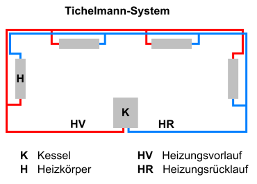
The reverse return, or Tichelmann loop, equalises the total developed length (outgoing plus return) of each branch: the first branch on the outgoing is the last on the return. The static imbalance disappears by design, without adjustment. It is the reference solution when it is feasible; OVHcloud notes that it is not always the case in large installations, « as it requires space and support for a long and large pipe » (translation: because it requires space and supports for a long and large diameter pipe), and it is precisely here that a branch control valve is used (D3). Note that the reverse return addresses the static imbalance, but not the dynamic coupling: it equalises the paths without making them insensitive to the total flow.
The ring topology, supplied at two points, acts on both fronts: it halves the flow carried by each section, thus the distribution pressure loss, and reduces the gap between the best and worst positioned take-offs. It constitutes a common architecture for large secondary loops.
2.2 Lever 2: pump regulation
This is the lever that validates the argument of § 1.2, and it deserves to be explained as it is too often taken for granted.
A fixed-speed pump does exactly the opposite of what is desired. Its characteristic curve decreases: when the total flow decreases, the manometric head increases. The closure of a branch therefore applies more pressure to the others, which then draw more flow than expected. The figure below quantifies the effect on a four-branch network.
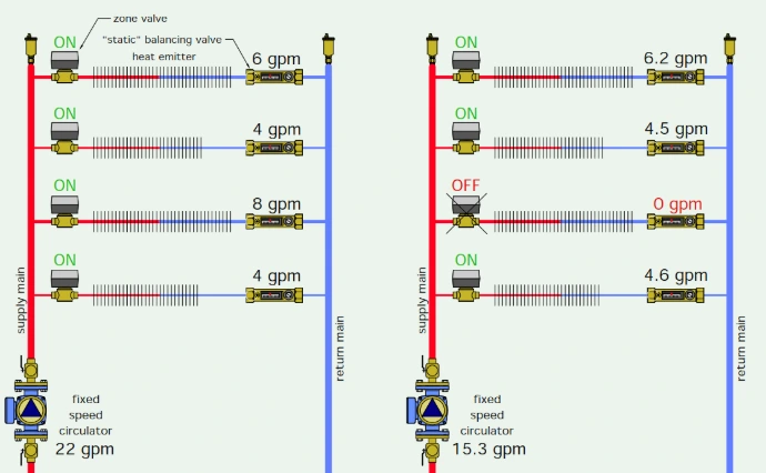
This textbook case serves to justify independent pressure limiters and is regularly presented as general proof. It is not: it assumes a fixed-speed pump. With a pump regulated on Δp, the residual drift is no longer that of the pump curve but only that of the distribution pressure loss, namely the term α / 2 of § 1.2, an order of magnitude lower.
The measurement point of the Δp is the only discrete choice that determines the quality of the result. Three strategies coexist:
- Measurement at the source. The simplest solution, adopted by most prefabricated units. The Δp is maintained upstream of the collectors, so the branches experience the full variation of Δpdist. This is the case covered by the criterion of § 1.2.
- Remote measurement at the disadvantaged point. The sensor measures the pressure at the last take-off. The term Δpdist cancels out for the furthest branch and changes sign for the others: the regulation then overestimates the pressure instead of underestimating it. The coupling becomes negligible, at the cost of a wired remote sensor.
- Sliding setpoint, where Δpset is recalculated from the total measured flow in order to analytically compensate for the distribution pressure loss. No remote sensor, but a hydraulic model embedded in the regulation.
2.3 Lever 3: the branch balancing device
The same valve body can belong to two different families depending on whether it has an actuator or not, which explains a large part of the terminological confusion. The table below sets the terms.
| Device | Principle | Flow Law | Actuator |
|---|---|---|---|
| Orifice Plate (flow setter, flow adjustment device) Fixed Resistance |
A calibrated, non-adjustable orifice, sized from the design stage. | ṁ ∝ √(Δp), Kv non-adjustable. No measurement without external instrumentation. | None |
| DRV (Double Regulating Valve, double adjustment valve) Manual balancing valve, known as static |
An adjustable orifice, set once at commissioning, with pressure taps to measure the flow. | ṁ ∝ Kv √(Δp), with Kv fixed. The flow follows every variation in network pressure. | None |
| PIBV (Pressure Independent Balancing Valve, pressure independent balancing valve) Pressure independent flow limiter |
Mechanical presetting of the flow and internal regulator of Δp (diaphragm and spring). The preset flow is maintained despite variations in the network. | ṁ = ṁpreset constant as long as Δp remains within the operating range. Otherwise, return to Kv √(Δp). | None, adjustment button only |
| PICV (Pressure Independent Control Valve, pressure independent control valve) = PIBV + actuator |
The same body, plus a motorised control element driven by an external controller (temperature, power). | ṁ = y · ṁpreset, where y is the control from 0 to 100%, independent of Δp. | Actuator, on/off, 3 points or 0-10 V |
| Smart valve (connected) |
Integrated measurement of flow, temperature and pressure, electronic regulation, feedback of BACnet or Modbus information. | Flow controlled to a setpoint in closed loop on the measurement. Pressure independence achieved electronically. | Actuator + electronics |
| DPCV (Differential Pressure Control Valve, differential pressure control valve) Δp branch regulator |
Maintains constant differential pressure across an entire branch, not the flow of a single terminal. | Does not fix the flow: it stabilises the Δp applied to downstream devices. | None |
Terminology. The two central families, PIBV and PICV, correspond physically to the same product; only the actuator distinguishes them. Caleffi indicates this unambiguously for its valve 145: « With the green manual adjustment knob as shown, this valve is an adjustable PIBV […] Adding an actuator changes the valve from an adjustable pressure-independent balancing device, to a pressure-independent control valve (PICV) » (R1, p. 25 and 26). Translation: with the green manual adjustment knob, this valve is an adjustable PIBV; adding an actuator transforms it into a pressure-independent control valve, that is to say a PICV. Common synonyms for the PIBV: automatic balancing valve, dynamic balancing valve. However, be careful with the acronym PIBCV (Pressure Independent Balancing and Control Valve) : despite the « B », it refers to the motorised, synonymous with PICV at IMI, FlowCon and Danfoss (R3). On the DLC side, OCP uses a simpler nomenclature: manual valves, automatic valves, control valves and (intelligent) valves compatible with telemetry (D2).
2.4 Inside a pressure-independent valve
Two functions are mounted in series in the same body (R1, R2), with the inlet on the left at p1, the outlet on the right at p3 and an intermediate chamber at p2.
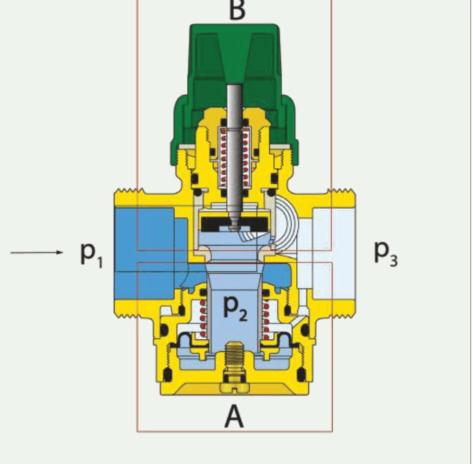
- the frame A, at the bottom, is stage 1: a movable valve connected to a diaphragm that sees p2 on one side and p3 on the other, held by a spring. It closes further as the pressure in the system increases, thus maintaining p2 − p3 constant (R2) ;
- the frame B, at the top, is stage 2: the rod and its valve reveal more or less a profiled orifice. This is where either a manual button (PIBV) or an actuator (PICV) operates, and where the maximum flow is preset.
The flow therefore only depends on the section opened by stage 2, and not on the system. Note that no position index is readable, unlike a manually balanced valve adjusted by the number of turns from a measured flow.
Figure 4: section of a PICV, with the two stages in series. Source: R1, figure 5-2.
The operating range constitutes the limit. Independence from pressure is only ensured between a Δp minimum and a Δp maximum at the valve terminals. Below the threshold, the valve becomes a simple orifice again and the system returns to the coupled regime, without any particular indication.
| Quantity | Value | Source |
|---|---|---|
| Δp minimum, small diameters | 16 kPa (DN 10 to 20), 20 kPa (DN 25), up to 35 kPa in high flow versions; 25 to 30 kPa for the Caleffi 145 DN 20 to 32 | R2, R1 § 5 |
| Δp minimal, large diameters | approximately 28 kPa (1½" to 10") | R2 |
| Below the threshold | « If there is not enough differential pressure the valve cannot reach the set flow ». Translation: without sufficient differential pressure, the valve cannot reach the set flow and reverts to an orifice at Kv √(Δp) | R2 |
| Δp maximum | 400 kPa (Caleffi 145: 60 psi, 414 kPa), 600 kPa (AB-QM threaded) | R1, R2 |
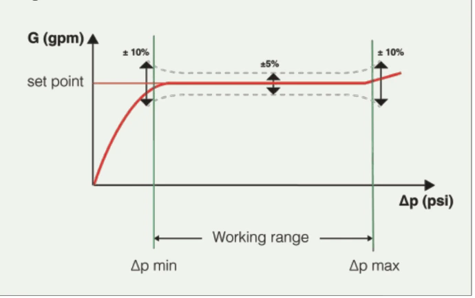
Two consequences follow. A pressure-independent device consumes its Δp minimum, 25 to 35 kPa depending on the range, drawn from the available manometric height: this hydraulic cost is not negligible. It also contributes nothing in scenarios of pressure loss, specifically those studied in transient conditions, since below the threshold it stops regulating and the flow collapses like with a passive device. Finally, the diaphragm cartridge is a moving part of small section, thus sensitive to fouling.
3. The heating of buildings, the origin of these devices
Each device in the table above was invented for buildings, and it is worth understanding why: these reasons are precisely what a data centre designer must confront in their own case.
The first case is the oldest : a boiler and a set of radiators in parallel on two pipes. The nearby radiators heat, while the distant ones remain cold. The historical fix is the simplest possible application of the branch law: a balancing valve on each radiator return, set once and then forgotten, which corresponds exactly to the DRV of § 2.3. Its modern industrial form, an adjustable orifice with two pressure taps and a preset index, remains the common device of the trade (R4). European practice considers this adjustment as part of the work, not as an optional refinement: EN 14336, the standard on the installation and commissioning of water heating systems, dedicates an annex to good practices for balancing water flows (B1).
Then the terminals began to modulate. Thermostatic valves, then two-way control valves of fan coil units, transformed each branch into a variable resistance controlled by the room. This results in four characteristics that make building hydronics difficult:
- The network is never at a single operating point. The total flow continuously oscillates between almost zero and full load; Δpdist therefore varies with it and the adjustment made at commissioning is only accurate for a single load.
- The diversity is great. A south facade closes while a north facade opens; the flow taken by part of the building is not correlated to that of the rest.
- The distribution is long and of small diameter. The rising columns are sized just right, so α is high and the coupling is first order, not a correction.
- The excess flow is costly. An excessive flow in a partially loaded emitter returns water that is too hot, which degrades the temperature difference of the system and the efficiency of pumping. In chilled water systems, this is the classic low delta-T syndrome, which Taylor largely attributes the causes and remedies to regulation and balancing defects (B2).
The industry has mobilised the three levers in order : first differential pressure control valves by rising column, which stabilise the Δp applied to a group of terminals (lever 2, applied locally), then pressure-independent balancing valves, which make each terminal indifferent to the pressure applied to it, and then the PICV, which combines balancing, regulation, and shut-off in a single body and eliminates any measurement at commissioning. The idronics 34 from Caleffi presents this evolution family by family (R1). The PICV therefore constitutes the right answer for a network where levers 1 and 2 cannot be pushed far enough.
This context should not be blindly transposed. The demonstration of figure 3, often used to justify pressure-independent valves, assumes a fixed-speed pump supplying modulating terminals. With a pump regulated on Δp and fixed terminal flows, the same figure loses much of its significance.
4. Liquid cooling in data centres
4.1 Why DLC is the favourable case
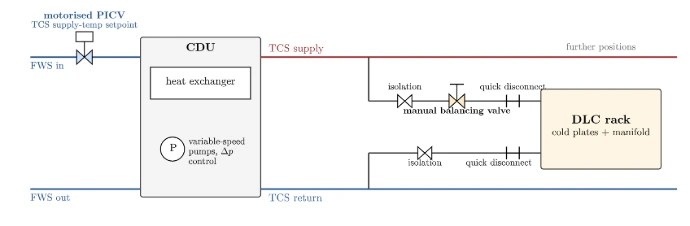
A DLC network is hydraulically identical to figure 1: a CDU between the facility water system (FWS, Facility Water System) and the technology cooling system (TCS, Technology Cooling System), two headers and a branch per rack including cold plates, hoses and quick connectors. But each of the characteristics from § 3 is reversed.
| Trait | Building heating | DLC |
|---|---|---|
| Branch flow | Module continuously according to the room | Fixed at sizing, about 1.5 L/min per kW; it is the temperature of departure that ensures regulation (D2) |
| Branch states | Continuum from 0 to 100 % | Only two: in service or isolated |
| Branch pressure loss | Moderate, dominated by the emitter | High, the cold plates are microchannels, so α is naturally small |
| Sizing of the distribution | Uplift columns of small diameter, sized as tightly as possible | Oversized to limit speed and maintain cleanliness, below 1.0 m/s (D4) |
| Source | Any pump, often fixed speed in older installations | Variable speed CDU pumps regulated on Δp, a specified requirement (D6) |
The last line is decisive. A CDU is by design a regulated source: the specifications require it to provide a « flow control », that is to « regulate and balance coolant flow delivered to racks or cooling manifolds » and to « maintain stable differential pressure under changing IT load conditions » (D6). Translation: regulate and balance the fluid flow delivered to the racks or manifolds, and maintain a stable differential pressure when the IT load varies. The OCP design guide explicitly outlines the resulting strategy:
« By understanding the total pressure drop and estimating the pressure loss within the supply and return pipes, the CDU’s pump speed can be regulated to deliver the required flow rate to each rack at the desired pressure. This target pressure drop serves as the setpoint for the entire system.
Adapting to changes in rack configuration: as racks are added or removed, the pump dynamically adjusts its speed to maintain the set pressure drop, thereby delivering the appropriate flow rate to meet the cooling demands of the connected racks.
Ensuring balanced flow: to prevent unbalanced pressures that may cause some valves to exceed their gauge limits at high flow rates, it is critical to regulate the flow to each rack. This is achieved using flow control valves installed on each branch. » D2Translation: by knowing the total pressure drop and that of the supply and return pipes, the speed of the CDU pumps can be regulated to provide each bay with the required flow at the desired pressure. This target pressure drop becomes the setpoint for the entire system. When adding or removing bays, the pump adjusts its speed to maintain this setpoint and provide the corresponding flow. Control valves installed on each branch finally ensure the balancing of flows and prevent some valves from exceeding their pressure limits.
This is, word for word, the diagram of § 1.2: a setpoint Δp at the system level, automatic adaptation to the number of bays, and a branch adjustment device whose role is limited to setting a resistance.
4.2 When a manual valve is sufficient
Three conditions, which are exactly the assumptions of § 1.2.
| Condition | Why | How to verify it |
|---|---|---|
| C1. The branch flow is not modulated | A manual valve fixes a resistance, not a flow. A terminal that must modulate its flow with the load requires a controlled device. | In DLC, the bay flow is fixed to the sizing and the cooling is controlled by the supply temperature. Condition satisfied. |
| C2. Δp is regulated at the source | Without this regulation, the pump curve transfers the pressure to the remaining branches (figure 3) and the coupling becomes first order. | Standard requirement of the CDU (D6, D2). Check the measurement point and the presence of group regulation. |
| C3. The branch authority is high | This is the criterion α ≤ 2ε. It limits the drift of the flow when the configuration changes. | Calculate the distribution pressure drop at maximum flow and relate it to Δp of a branch. Target α ≤ 10 %, reference 1/40 (D4). |
Once balanced, such a network remains balanced. This is precisely OVHcloud's argument for the manual valve: it is suitable for « large installations with server racks […] where the configuration of the racks to be installed is well-documented over a period », when « the pressure drop is precisely defined based on the cooling circuit within the rack » and « the system can be simulated or tested before the final deployment » (D3). Translation: it is suitable for large installations where the configuration of the racks and the pressure drops are well defined, and which can be simulated or tested before final deployment. OCP cites manual valves as a valid flow adjustment option (D2) and its recommendations for connecting to the racks extend to a configuration « double isolation valve + grooved coupling », consisting of two isolation valves and a grooved coupling. The document specifies that « double ball valves enable use of vent / drain / bypass connections to address commissioning and onboarding challenges as well as flow stabilization » (D2), meaning that two ball valves allow for the necessary purge, drain, or bypass connections for commissioning and flow stabilization. The branch device can therefore be a manual balancing valve of the IMI TA or STAD type (a DRV with pressure taps), or even a marked isolation ball valve. Pressure taps are essential, as they allow the commissioning team to measure and adjust the flow, unlike a pressure-independent cartridge.
4.3 When this is not enough
Four situations invalidate the previous conditions and justify a pressure-independent or intelligent valve:
- Long, branched, or undersized collectors, therefore α greater than 10%. A typical case is a branch in DN 25 (1"): at identical power and bay flow, OCP indicates that its pressure drop can reach five times that of a DN 50 (2") pipe (D2). The distribution then consumes a significant portion of the Δp available and the branches reconnect.
- Large disparity of power between racks on the same distribution, a situation explicitly addressed in the MCV white paper as a branch balancing case (D3).
- Gradual deployment. Between the delivery of the network and the occupation of all locations, the total flow varies greatly. The current solution is not a PICV, but a compensating bypass : OCP recommends the « incorporation of a regulating valve into the bypass connection to impose a false resistance equivalent to that of the rack + manifolds » (D2), that is, a regulating valve on the bypass imposing a resistance equivalent to that of the rack and its collectors. This allows for the validation of the CDU flow and for pre-setting the valves before the actual arrival of the racks.
- Need for telemetry by rack. A manual valve does not transmit any flow measurement. If this flow is to become a monitored point, a flow meter or an intelligent valve becomes necessary.
4.4 What the DLC references say
There is no prescriptive standard for balancing a TCS loop, but a set of now converging guides.
| Document | Contribution to balancing and regulation |
|---|---|
| D1 ASHRAE TC 9.9 Liquid Cooling: Resiliency Guidance for Cold Plate Deployments, 2024 |
Framing document. It places the CDU at the FWS / TCS interface, requires an active redundancy of the pumps, recommends the « transient modeling of the TCS/FWS systems », that is to say a transient modelling of the TCS and FWS systems, as well as hydraulic and thermal commissioning. Notable result: up to 27 °C of TCS temperature jump during a pump switch without active redundancy. |
| D2 OCP Modular TCS at Cloud Scale: Design, Delivery & Selection Guidance, Rev 1, 2025 |
The most directly useful document. Setpoint strategy Δp at the system level, adaptation to the number of racks, one control valve per branch, manual / automatic / regulation / intelligent typology, comparison DN 25 against DN 50, a compensation bypass for gradual deployment, 25-micron filtration and commissioning according to ASHRAE Guideline 0. |
| D3 OCP White Paper: MCV (Manual Control Valve), A. Chehade, OVHcloud, 2023 |
Argument in favour of the manual valve on a TCS loop, described as « a replacement for an automatic regulation valve used for flow distribution adjustments », that is to say a replacement solution for an automatic regulation valve to adjust flow distribution. Three cases: large installations without a Tichelmann loop, longitudinal disparity, vertical disparity. |
| D4 LBNL and working group Open Specification for a Liquid Cooled Server Rack |
Quantified criteria: collector speed less than 1.0 m/s, pressure drop in the collector less than one fortieth of that of a computer loop, maximum deviation of 10%, beyond which balancing valves are required. Source of the authority criterion of § 1.2. |
| D5 OCP Guidelines to Rack Manifold Requirements and Qualification, v3 |
Same issue at the bay collector scale: uniform distribution to each server, speed less than 1.5 m/s, vent at the high point, drain at the low point, and local adjustment devices for CDU end-of-row architectures. |
| D6 OCP CDU Performance & Specification Guidance for Modular TCS |
Expected role of the CDU: regulate and balance the flow supplied to the racks, maintain a Δp stable under variable computer load, ensure N+1 or 2N redundancy with automatic failover, and allow for testing and integration into the BMS. |
Two cross-cutting observations. First, none of these documents prescribes a type of valve: all refer to a case-by-case analysis, and D2 indique que « the pros and cons of control methodologies (manual, automatic & use of telemetry) is a complex discussion beyond the scope of this paper », soit que les avantages et les inconvénients des méthodes de régulation manuelles, automatiques ou par télémétrie dépassent le cadre du document. Deuxièmement, tous convergent vers la nécessité d’un modèle hydraulique du réseau, que ce soit pour la modélisation transitoire requise par D1, the pre-deployment simulation recommended by D3, or the « transfer of hydraulic models to support future planning » requested during commissioning by D2, that is, the transfer of hydraulic models intended to support future developments.
5. The impact on the modelling of balancing systems
At SIL3X, we specialise in the dynamic modelling of energy systems. The same equations apply for distribution to local cooling units in nuclear and for a data centre DLC loop: a source (CDU or group), a distribution network, parallel branches, and a flow setpoint or Δp to be maintained under variable load.
The right level of model. Several representations are possible. The criterion is not sophistication, it is the question to be addressed. A model that is too simplistic misses the phenomenon (authority, pump switching, thermal front). A model that is too rich, compressible, inertial, meshed beyond necessity, makes the calculation too slow to simulate the entire loop, the redundancies, and the commissioning scenarios. One does not use a hammer to kill a fly: one chooses the smallest set of equations that captures the quantities of interest, in order to maintain numerical performance compatible with the entire network (D1, D2, D3).
Three levels cover the essentials of balancing and regulation studies.
1. Simple thermal, imposed flows. Energy balance on volumes, heat exchangers, and racks, with prescribed flows (nominal, or from a scenario). This is the fastest model: it allows for the representation of the entire loop, IT powers, supply and return temperatures, and the thermal sizing of the CDU. Its limit is structural: without a hydraulic network, there is neither pressure, nor flow sharing, nor transient of Δp. It therefore cannot handle a pump switch, a branch closure, or an authority drift α, nor the effect of pressure losses from the CDU and the collectors on the pressure available at the bays. It remains suitable when the flow rate is an assumption, not an unknown.
2. Hydraulics (quasi-static or slow dynamic). Pumps, characteristics H(Q), valves (Kv), pressure losses from piping, collector and CDU, regulation of Δp or flow rate. This is the model requested by the guides: simulation before deployment (D3), transfer of hydraulic models for developments (D2), criterion α and 1/40 (D4). It becomes necessary as soon as the losses from the CDU, the heat exchanger and the collectors weigh on the pressure at the ends of the branches, thus affecting the actual flow rate delivered. It allows for the sizing of balancing valves, to check the setpoint Δp (D6) and to compare a manual valve to a PICV. Transport is not modelled, which makes the complex transients of electrical loss, chiller shutdowns and recovery by buffer tanks inaccessible.
3. Hydraulics and thermal transport. We add the transport of temperature fronts in the pipes (advection, fluid volumes, delays). This level is justified when the phenomenon of interest is a front (which quickly becomes the case with very large piping networks), and not just a flow rate: pump switching without active redundancy, mixing FWS / TCS, network length, or the temperature jump of TCS up to 27 °C cited by ASHRAE (D1). Without transport, a hydraulic model provides the flow rates immediately, but misses the delay and amplitude seen by the cold plates.
In practice, the three are often combined: imposed flow rates for an initial energy balance of the entire loop, hydraulic for balancing and CDU losses, transport only on the sections where volume and travel time matter. The model remains light enough to cover N+1, the gradual deployment and commissioning, while staying true to the quantities that the guides require to be checked.
5. Takeaways
- Balancing is an authority problem, not a valve problem. The determining number is α, the ratio between the distribution pressure loss and that of the branch; the maximum drift is α / 2.
- Three levers act and substitute: sizing and topology of the network, source regulation and branch balancing device. One must choose the least costly combination that respects the tolerance, not the most sophisticated valve.
- The pressure-independent valve was designed for building hydronics, where the terminals modulate, diversity is high and the risers are of small diameter. These characteristics must be verified before transposing the solution.
- In DLC, they are reversed. With a CDU regulated on Δp (D6) and collectors sized to maintain α below 10%, with 1/40 as a reference (D4), a manual balancing valve with pressure taps, or a marked isolation ball valve, is sufficient. This is the first option presented by OCP (D2, D3).
- A PICV or an intelligent valve remains relevant when the assumptions are not met: fixed speed pump, long or small diameter collectors, high power disparity between bays or telemetry requirement per bay.
- Whatever the choice, the sizing must be based on a hydraulic model and confirmed by a rigorous hydraulic and thermal commissioning (D1).
- The model follows the same logic as the valve: the smallest level that captures the phenomenon. Thermal at imposed flows for the balances, hydraulic as soon as the pressure and CDU losses count, transport of fronts only if thermal delays are at play. Too much fidelity prevents simulating the entire loop.
6. References
Figures 3, 4 and 5 come from issue 34 of idronics published by Caleffi (R1), an open access publication reproduced here with attribution for technical illustration purposes. It is the most comprehensive source on balancing valve families. Figure 2 is in the public domain (B3).
References and guides from the DLC industry
| D1 | ASHRAE TC 9.9, Technical Bulletin: Liquid Cooling, Resiliency Guidance for Cold Plate Deployments, September 2024, 4 p. Direct PDF : tpc.ashrae.org, FileDownload (PDF). Also listed under Other Publications on the TC 9.9 documents page: tpc.ashrae.org, TC 9.9 documents. Available in the Datacom Encyclopedia (datacom.ashrae.org, subscription). |
| D2 | Open Compute Project, Modular Technology Cooling System for Cloud Scale: Design, Delivery & Selection Guidance, Rev 1, 2025. D. Mitchell (Victaulic), V. Sorell (Oracle), H. Kabbani (Google), A. Chehade (OVHcloud), V. Prasad (Microsoft), P. Shahi (NVIDIA) et al. opencompute.org, Modular TCS Rev 1 (PDF) |
| D3 | Open Compute Project, White Paper: MCV (Manual Control Valve), A. Chehade, OVHcloud, December 2023. opencompute.org, white paper MCV (PDF) |
| D4 | Open Specification for a Liquid Cooled Server Rack, working group hosted by the Center of Expertise for Energy Efficiency in Data Centers, LBNL. datacenters.lbl.gov, Open Specification (PDF) |
| D5 | Open Compute Project, White Paper: Guidelines to Rack Manifold Requirements and Qualification, v3, B. Wondimu, E. Kung, D. Zhou (Intel) et al. opencompute.org, rack manifold v3 (PDF) |
| D6 | Open Compute Project, CDU Performance & Specification Guidance for Modular TCS, Data Center Facility group. ocp-all.groups.io, CDU performance guide (PDF) |
Heating of buildings and hydronics
| B1 | CEN, EN 14336:2025, Heating systems in buildings: installation and commissioning of water based heating and cooling systems (paid standard), with an informative annex on best practices for balancing water flows. Replaces EN 14336:2004, withdrawn in June 2025. standards.iteh.ai, EN 14336:2025 |
| B2 | S. T. Taylor, Degrading Chilled Water Plant Delta-T: Causes and Mitigation, ASHRAE Transactions, vol. 108, part 1, 2002, p. 641. Bibliographic notice IIR Fridoc 2003-1517 : iifiir.org, notice 20367 |
| B3 | Tichelmann System, diagram of a reverse return radiator loop, Kino, SVG redrawn by Marlus Gancher, 2011. Wikimedia Commons, public domain. commons.wikimedia.org, File:Tichelmann System.svg |
| B4 | Wikipedia, Tichelmann Loop. fr.wikipedia.org, Tichelmann Loop |

Manufacturer documentation
| R1 | Caleffi, idronics no 34, The Evolution of Hydronic Balancing Valves, January 2024, 40 p., open access. § 3 manual valves, § 4 PIBV from p. 19, § 5 PICV from p. 25. caleffi.com, idronics 34 (PDF) Web chapters : § 4 PIBV and § 5 PICV. |
| R2 | Danfoss, AB-QM, pressure independent balancing and control valve. Source of minimum and maximum values of Δp. Technical data sheet DN 10 to 250 : assets.danfoss.com, AI186586479945 (PDF) North American documentation, 1½" to 10" : assets.danfoss.com, AI194086469170 (PDF) |
| R3 | IMI Hydronic Engineering, PICV: TA-Modulator (use of the acronym PIBCV for the motorised version). climatecontrol.imiplc.com, TA-Modulator |
| R4 | IMI Hydronic Engineering, STAD, balancing valves DN 10-50, PN 25, technical data sheet. Manual balancing valve taken here as reference : Kvs DN 50 = 32.3 m3/h, presetting, measurement, isolation and draining functions. technical data sheet STAD PN 25 (PDF) |